
Low-noise preamplifier selection guide
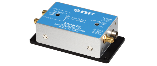
Differential input type
- Reliably amplify a wide range of voltage signals between sub-µV and several mV
- Lineup of models supporting a wide frequency range between DC and up to 500MHz
- The most suitable model can be selected according to the signal source resistance.
-
Information
-
Measurement example
Information
Lineup
| Input type | Gain | Bandwidth | Input resistance | Noise voltage density | Noise current density | Noise figure | |
|---|---|---|---|---|---|---|---|
| SA-410F3 | Differential input | 40dB | DC to 1MHz |
1kΩ/ 10kΩ/ 100kΩ |
0.75nV/√Hz | 4.5pA/√Hz | - |
| SA-420F5 | 46dB | 1kHz to 80MHz |
1MΩ | 0.9nV/√Hz | 100fA/√Hz | - | |
| SA-421F5 | 46dB | 30Hz to 30MHz |
1MΩ | 0.5nV/√Hz | 100fA/√Hz | - | |
| SA-430F5 | 46dB | 1kHz to 100MHz |
50Ω | 0.35nV/√Hz | 7pA/√Hz | 1.0dB | |
| SA-440F5 | 40dB | DC to 20MHz | 1MΩ/ 100MΩ/ OPEN |
1.8nV/√Hz | 25fA/√Hz | - |
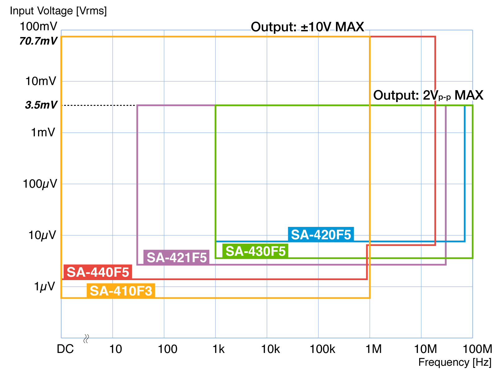
Input voltage - Frequency response
The model line-up supports a wide voltage input range. Includes extremely small voltages of less than 1 μV.
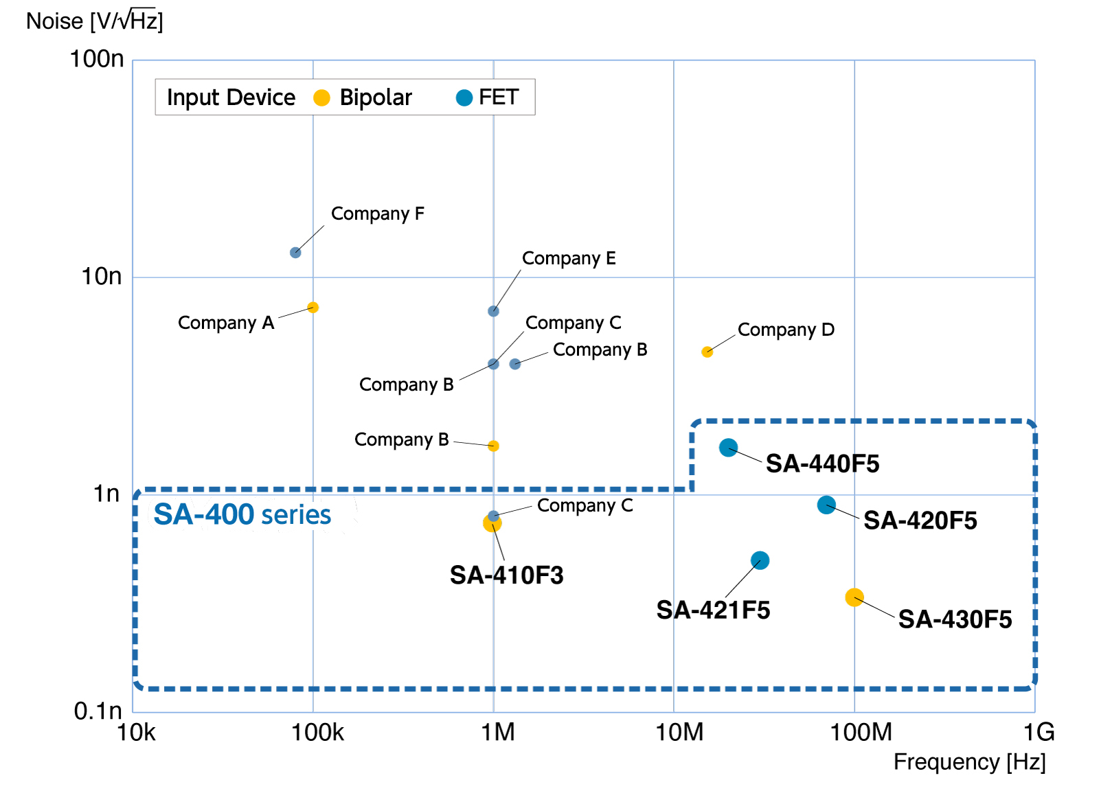
Output noise - Frequency response
Supports models with frequency ranges up to 100MHz. Achieves low noise specifications compared to competitors.
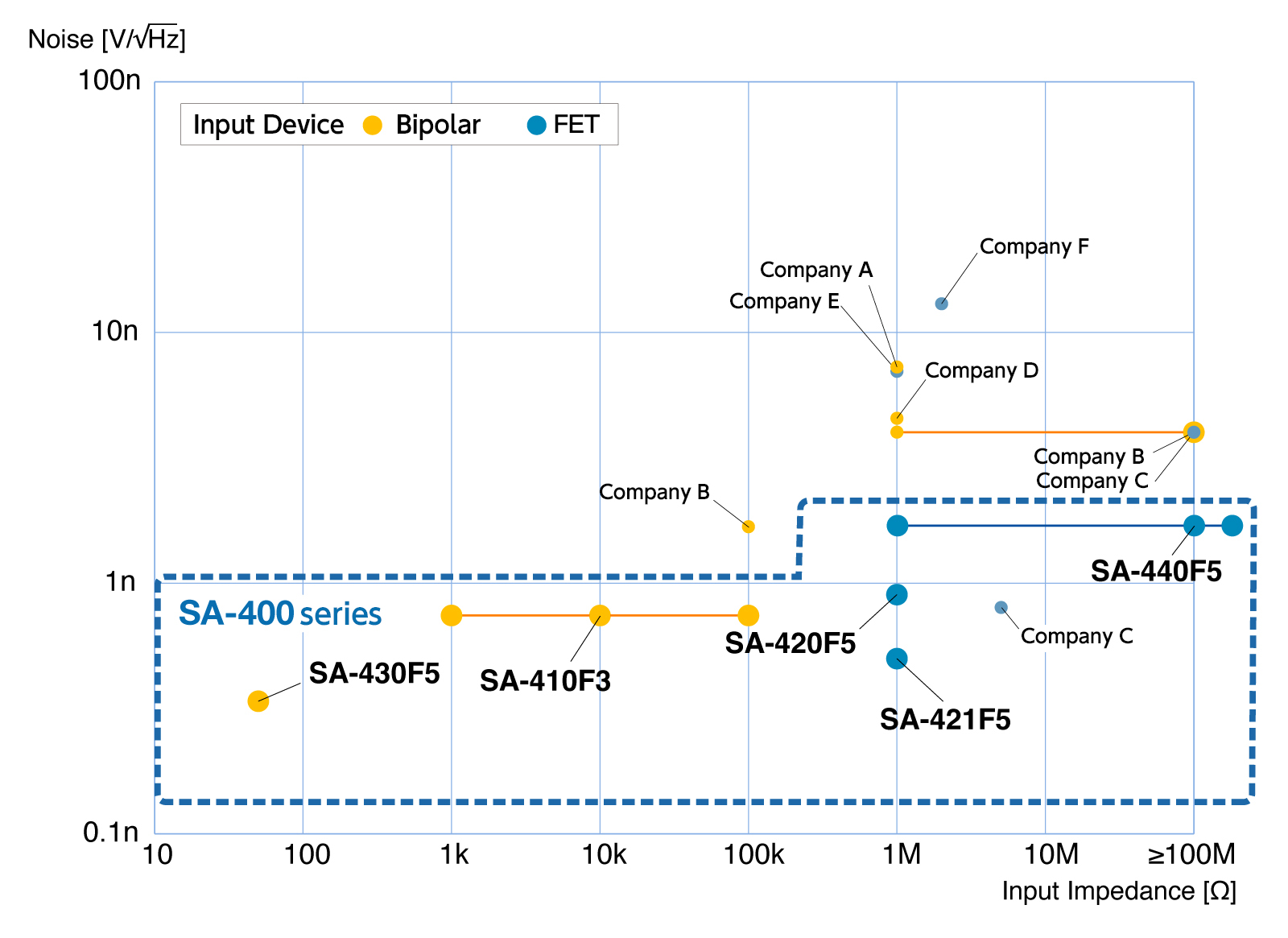
Output noise - Input impedance Characteristics
An amplifier suitable for the signal source resistance of the sensor can be selected. Achieves low-noise signal output.
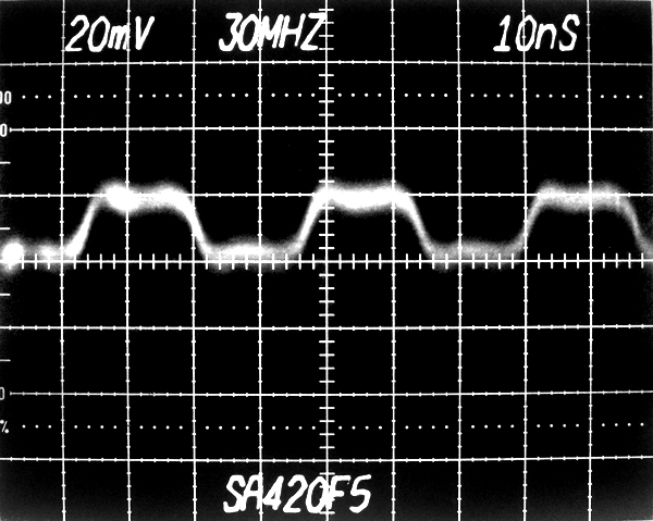
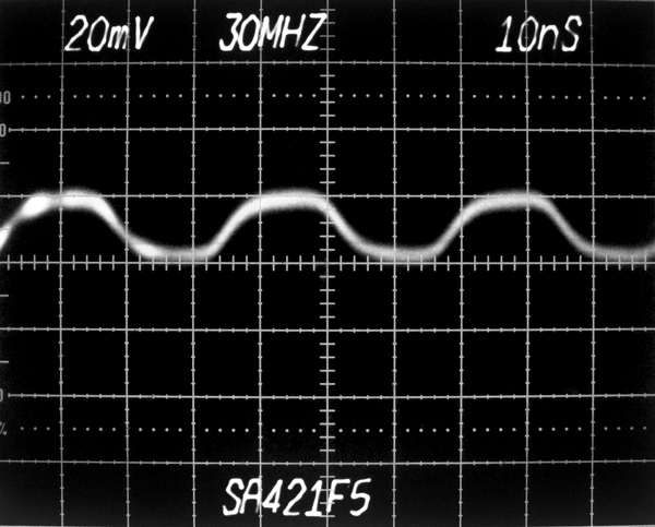
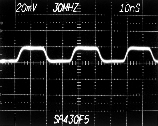
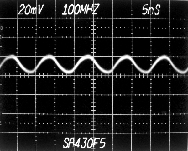
Pulse response
Output waveform comparison at 100μVp-p square wave input
SA-410F3 (DC to 1MHz, 0.75nV/√Hz)
SA-420F5 (1kHz to 70MHz, 0.9nV/√Hz)

SA-421F5 (30Hz to 30MHz, 0.5nV/√Hz)

SA-430F5 (1kHz to 100MHz, 0.35nV/√Hz)
SA-440F5 (DC to 20MHz, 1.8nV/√Hz)

Measurement example
Challenging the signal detection limit (µV real-time signal)
Small signals amplified by the SA series are observed with an oscilloscope.
SA-410F3
- Input signal: 5μVp-p, sine wave
- Oscilloscope: 1MHz bandwidth
- LPF: Connected after the amplifier and set a cutoff frequency about 5 times the signal frequency*
LPF=300Hz
LPF=3kHz
LPF=30kHz
LPF=300kHz
Detects 5µVp-p real-time signals
Waveform without LPF
*Using an appropriate LPF can reduce overall noise as shown above.
Challenging the signal detection limit (nV repetitive signal)
Connect multiple SA series units and observe using the averaging function of the oscilloscope.
Measurement block diagram
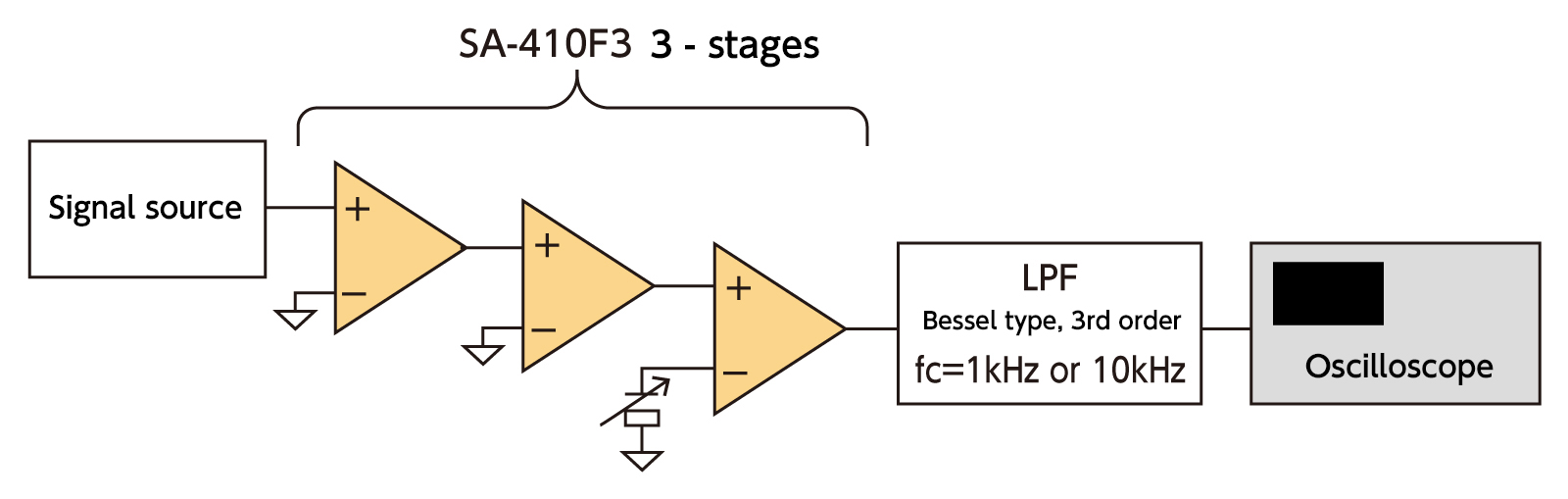
Measurement results
SA-410F3
- Input: 4nVp-p@55Hz, Pulse width: 1.82ms
- Measurement bandwidth: 1kHz
- Averaging process: 10,000 times
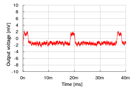
4nVp-p signal detected